
How does the brain see?
I’m interested in perception and signaling systems, particularly in humans. This post is a hodgepodge of various sources about visual processing models inspired by biological mechanisms. Back in undergraduate, I experimented with RNNs to predict dash camera misalignment, and although a basic model, it got me thinking about factoring objects into forms and transformations.
I bought the OpenBCI Gangelion board and some electrodes to monitor EEG signals from my brain, but with only 4 channels I won’t learn much. That will likely be a separate post.
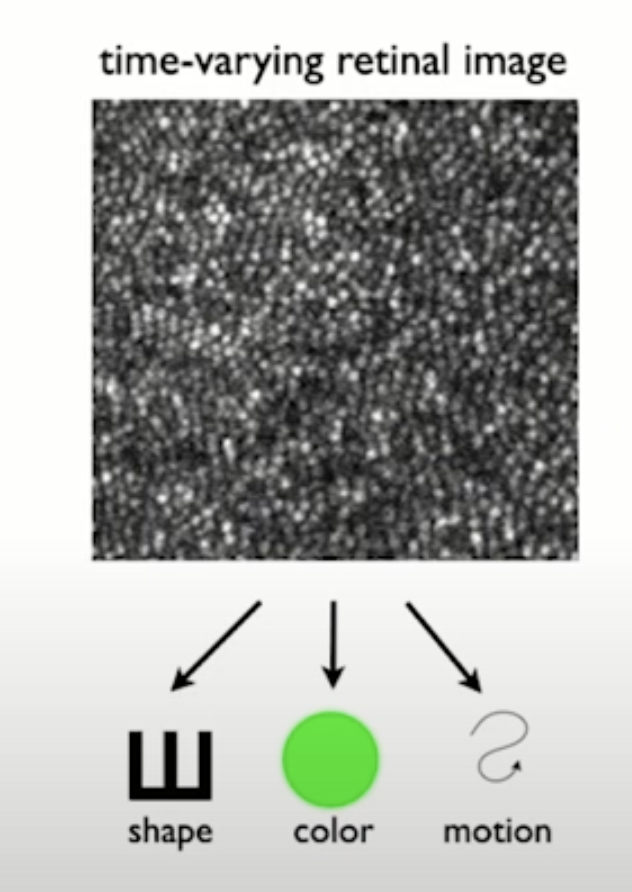
Photoreceptors send high-dimensional signals to ganglion cells of the retina. They filter noise and redundancy to collectively transmit image-forming and non-image forming visual information via activations to other brain regions. The cones on the back of the eye perceive scene information from the photoreceptors. The image ([1]) below depicts the separation of shape, color and motion from a scene. The visual cortex has to compute and represent geometric transforms (equivariance) and recognize shapes independent from variations in pose, motion or lighting (invariance).
A pattern reaching the photoreceptors is compressed by retinal circuits to a single spike of the ganglion neuron cell (Chapter 11 [3]). Mathematically, how can these spikes relate to embeddings of objects and transforms? Below I reproduce a digram from [1] explaining how a pattern maps to a unique point on a manifold. The set of points live on nonlinear manifold. The halfway point corresponds to a superposition of both patterns at half contrast so manifold has to be curved.
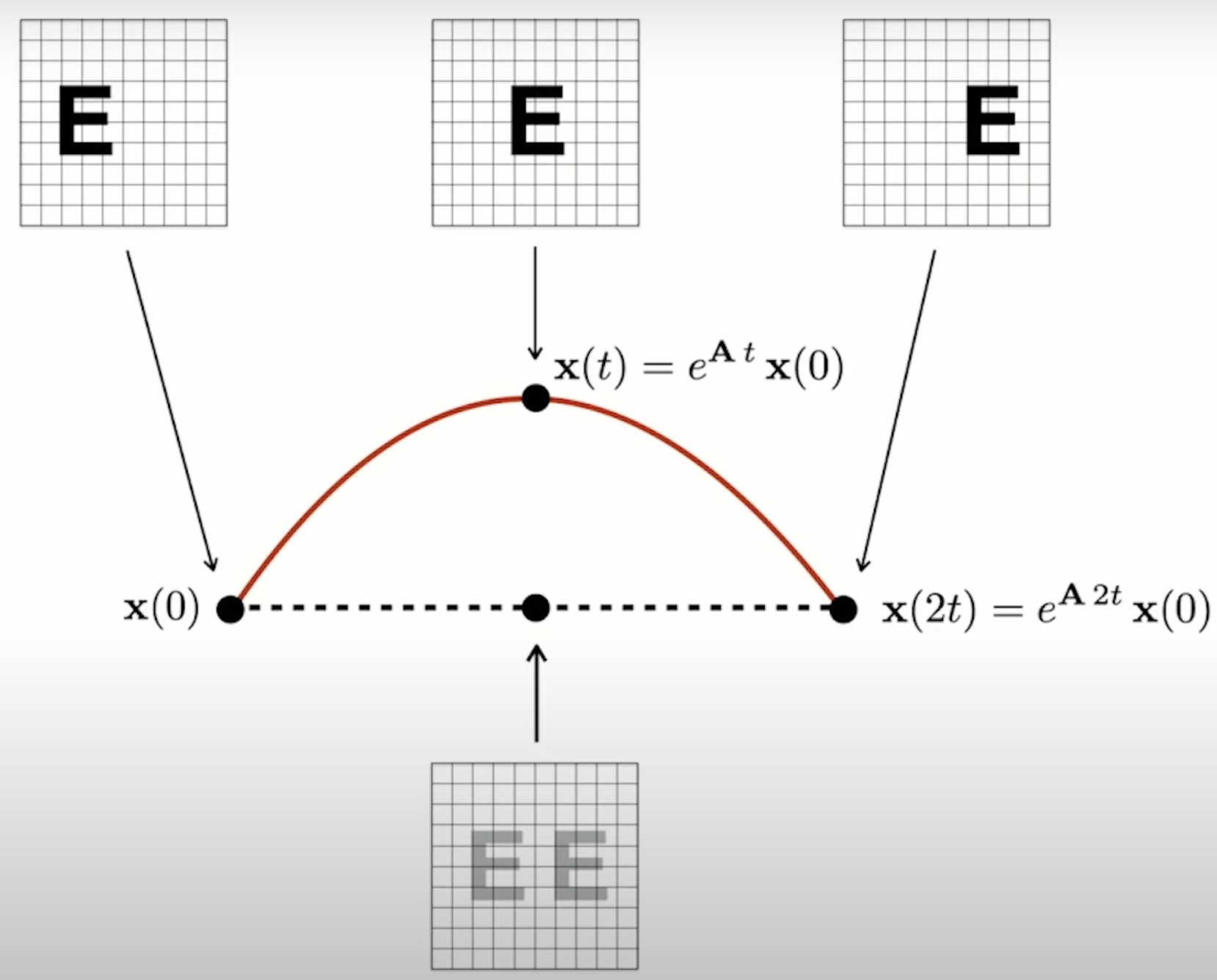
The theory of Lie groups says all matrices moving on this manifold belong to same group. Different patterns trace out different manifolds but importantly the Lie operator is the same. Some other examples include the groups of n-dimensional rotations SO(n) (special orthogonal) and rigid motions SE(n) (special Euclidean). Images can be explained as the product of transformations on shapes. It is reminiscent of Plato’s theory of forms, where physical objects are merely imitations of the non-physical ideas.
Formally, [2] combines Lie Group transformation learning and sparse coding within a Bayesian model. The images become a sparse superposition of shape components followed by a transformation that is parameterized by continuous variables. The generative image model is $$ I = T(s) \Phi\alpha + \epsilon $$
- transformation parameter s is a random vector with i.i.d elements
- dictionary $\Phi$ with each column having unit L2 norm
- sparse code $\alpha$ is a random vector with i.i.d elements draw from an exponential distribution
- random noise $\epsilon$ is i.i.d.
The transformations T(s) are parameterized as actions of compact, connected, commutative Lie groups on images. They can be decomposed using Peter-Weyl theorem to get $$ I = e^{A s}\Phi\alpha + \epsilon $$ $$ I = We^{\sum s}W^T \Phi\alpha + \epsilon $$ $$ I = WR(s)W^T \Phi\alpha + \epsilon $$
- R(s) is the learned block diagonal matrix of complex phasors.
- W is learned orthogonal matrix of the transform group
This imposes theoretical constraints on learnable transformations, but they can still be approximately learned in practice.
- Compactness enforces the transformations to be periodic
- Connectedness precludes discrete transformations like reflections
- Commutativity excludes non-commutative transformations such as 3D rotations
The block diagonal structure allows for efficient inference and learning. Reformulate as vector factorization. Can’t gradient descent because of too many local minima. Instead, perform gradient ascent on log-likelihood $$ W^TI = R(s)W^T \Phi\alpha + \epsilon $$
$$ \overset{\sim}{I} = z(s) .* \overset{\sim}{O}(\alpha) $$
- equivariant part z(s) is diagonal elements of R. Elements are complex phasors
- invariant part O(\alpha) is shape model
The learning update is $$ \nabla_{\theta} \ln P_{\theta}(\mathbf{I}) \approx \mathbb{E}{s \sim P{\theta}(s | \mathbf{I}, \hat{\alpha})} \left[ \nabla_{\theta} \ln P_{\theta}(\mathbf{I} | s, \hat{\alpha}) \right] $$
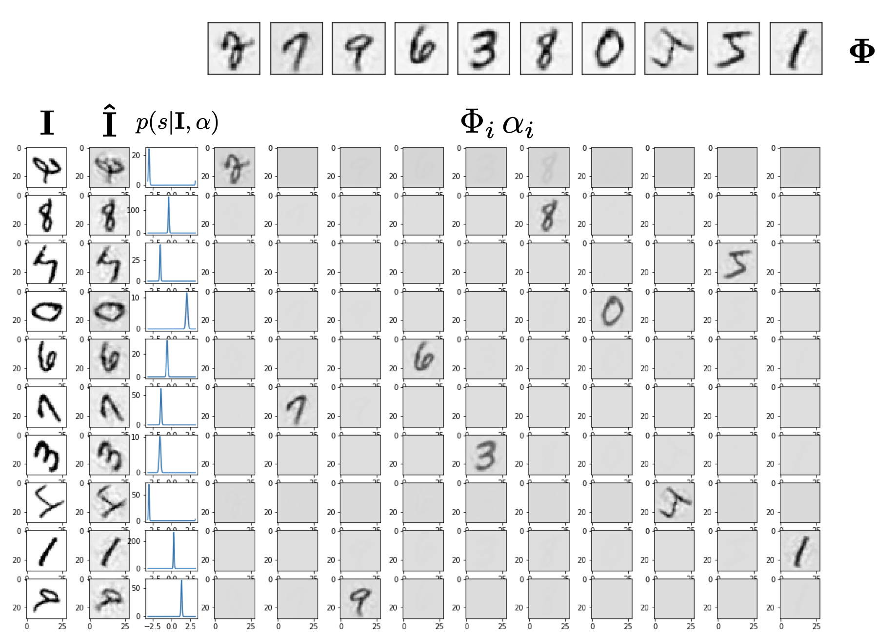
The paper uses a Riemannian ADAM optimizer. The set of values {x} can be represented in weighted superposition. We get sum(N) representational complexity instead of product(N). Here I reproduce the figure from [2], showing the method applied to MNIST digits.
Future reading:
- Section 2.6.2 [7] covers exact solutions to the subset sum problem. How could this be extended to quantum applications using residue numbers? I’ve just seen factoring papers.
References
[1] Invariance and equivariance in brains and machines
[2] Disentangling images with Lie group transformations and sparse coding
[3] Principles of Neural Design
[4] Analog Memory and High-Dimensional Computation
[5] Neuromorphic Visual Scene Understanding with Resonator Networks
[6] Hippocampal memory, cognition, and the role of sleep
[7] Computing with Residue Numbers in High-Dimensional Representation
[8] Visual scene analysis via factorization of HD vectors