Towards optimal annealing of oscillator networks for combinatorial optimization

This is an informal explaination of my unreleased paper analyzing Kuramoto dynamics for combinatorial optimization. It’s the optimal control theory of the experimental circuit I built previously. The connections to Morse theory follow from my conversations with Cleve Moler and Indika Rajapakse.

Disclaimer: The following text is an adapted AI summary of the paper.

The setup: oscillators that solve optimization problems

An oscillator-based Ising machine encodes a combinatorial problem in the phases of coupled oscillators. Each oscillator has a phase $\theta_i$. The problem lives in a symmetric coupling matrix $J$. A second-harmonic injection signal (“locking”) pushes every phase toward either $0$ or $\pi$, and those two values are read out as spins.

In a frame rotating with the injection reference, the Ising–Kuramoto (IK) dynamics are

$$ \dot\theta_i=-K_c\sum_{j\ne i}J_{ij}\sin(\theta_i-\theta_j)-K_s\sin(2\theta_i), $$

where $K_c$ is the coupling strength and $K_s$ the locking strength. These dynamics are gradient descent on the torus, $\dot{\boldsymbol\theta}=-\nabla E$, with potential

$$ E(\boldsymbol\theta)=-K_c\sum_{i<j}J_{ij}\cos(\theta_i-\theta_j)-\frac{K_s}{2}\sum_i\cos(2\theta_i). $$

So $E$ can only go down: $dE/dt=-|\nabla E|^2$. At a binary configuration, with $x_i=\cos\theta_i\in{\pm1}$, the potential becomes the Ising energy plus a constant:

$$ E(\boldsymbol\theta_{\boldsymbol x})=K_cH(\boldsymbol x)-\frac{NK_s}{2},\qquad H(\boldsymbol x)=-\tfrac12\boldsymbol x^{\mathsf T}J\boldsymbol x . $$

That constant is the catch. Every binary configuration is an equilibrium, good or bad. What separates a useful readout from a useless one is whether the dynamics can actually settle there. That depends on the landscape’s curvature, which is the subject of the paper.

Only the ratio $\rho=K_s/K_c$ matters for which equilibria exist and whether they are stable. From here on $K_c=1$ and $K_s=\rho$.

Curvature, stability, and the Morse index

The Hessian of $E$ is

$$ B_{ij}=\begin{cases} \displaystyle\sum_{k\ne i}J_{ik}\cos(\theta_i-\theta_k)+2\rho\cos(2\theta_i), & i=j,\[4pt] -J_{ij}\cos(\theta_i-\theta_j), & i\ne j. \end{cases} $$

At an equilibrium the Jacobian is $-B$, so the eigenvalues of $B$ settle linear stability:

• All positive: a strict local minimum, which attracts nearby trajectories.
• Some negative: a saddle. The number of negative eigenvalues is the Morse index $k$, the number of directions a trajectory can escape along.

The Morse index is the landscape’s bookkeeping. It says which stationary points could possibly be attractors ($k=0$) and how unstable the rest are.

Three kinds of equilibria (Cheng et al.)

Cheng et al. sort IK equilibria by their phase configuration. The paper uses that classification, extended to weighted, signed couplings.

Type I: binary or quadrature. All phases are in ${0,\pi}$, or all are in ${\pi/2,3\pi/2}$. These stay equilibria no matter how the gains change.

• For a binary state, define the gauged weights $w_{ij}=J_{ij}x_ix_j$. Split them into satisfied ($w>0$) and frustrated ($w<0$) edges, with graph Laplacians $L_+$ and $L_-$. The Hessian is then $B=L_+-L_-+2\rho I$. The state is stable when $$ \rho>\frac{\lambda_{\max}(L_–L_+)}{2}. $$
• Quadrature states always have the negative eigenvalue $-2\rho$ in the uniform direction, so they are never attractors.

Type II: mixed quadrant phases. Some phases are binary and some are quadrature. These are always unstable. For Gaussian couplings they also need exact cancellations, so they occur with probability zero.

Type III: everything else (non-quadrature). These are stable exactly when $\lambda_{\min}(B)>0$.

Attraction-domain estimates

Stability says a state attracts something; an attraction-domain estimate certifies how much. Both estimates use the Lyapunov function $V=|\boldsymbol\theta-\boldsymbol\theta^*|^2$ and certify a ball around the equilibrium.

For a binary state, the ball of radius $\beta\pi/2$ is certified whenever

$$ Q_\beta=2L_–2\frac{\sin(\beta\pi)}{\beta\pi}\big(L_++2\rho I\big)\prec 0,\qquad 0<\beta<1 . $$

There are two good sanity checks:

• As $\beta\to0$, $Q_\beta\to-2B$. So any strictly stable binary state gets some positive certified radius.
• If there are no frustrated edges ($L_-=0$), every $\beta<1$ works, and the ball has radius $\pi/2$.

Dropping the favorable $L_+$ term recovers Cheng’s original, more conservative condition.

For a stable Type III state, a Taylor-remainder argument certifies the radius

$$ r_A=\frac{\lambda_{\min}(B)}{2N,(d_{\max}+2\rho)},\qquad d_{\max}=\max_i\sum_{j}|J_{ij}| . $$

In both cases the key quantity is the bottom of the Hessian spectrum. That motivates the main tool of the paper.

Predicting the whole spectrum with a resolvent

Diagonalizing one Hessian is easy. Understanding how the spectrum of a whole population of equilibria depends on $\rho$ is harder. The paper adapts a random-matrix approach from Yamamura, Mabuchi and Ganguli. The idea:

1. Keep the diagonal. $B_{ii}$ holds all the information about the phases and the locking, so it stays exact.
2. Randomize the off-diagonals. Replace each coupling $-J_{ij}\cos(\theta_i-\theta_j)$ by an independent Gaussian with the same variance. For Sherrington–Kirkpatrick (SK) couplings, $J_{ij}\sim\mathcal N(0,1/N)$, that variance is $$ C_{ij}=\frac{\cos^2(\theta_i-\theta_j)}{N}. $$

The phase dependence of $C_{ij}$ is the IK-specific ingredient. Oscillator pairs 90° apart are decoupled in the Hessian.

For a matrix with this structure, the diagonal entries of the resolvent $R(z)=(B-zI)^{-1}$ satisfy the vector Dyson equation:

$$ \widehat R_{ii}(z)=\frac{1}{B_{ii}-z-\sum_j C_{ij}\widehat R_{jj}(z)} . $$

Solving this self-consistently gives the predicted eigenvalue density

$$ P_\eta(\lambda)=\frac{1}{\pi N}\operatorname{Im}\sum_i\widehat R_{ii}(\lambda+\mathrm i\eta), $$

and the Morse index is just the weight below zero:

$$ \frac{k}{N}=\int_{-\infty}^{0}P(\lambda),d\lambda . $$

Three populations of equilibria

The paper applies the resolvent to three populations, sampled numerically at $N=100$ over four SK instances.

Typical critical points

These are the most common stationary points: the most populated Morse-index class, then its most populated energy bin. At strong locking their phases crowd toward multiples of $\pi/2$, and the Hessian splits cleanly into two groups:

• Binary phases ($0,\pi$): diagonal near $+2\rho$.
• Quadrature phases ($\pi/2,3\pi/2$): diagonal near $-2\rho$.

Couplings between the two groups vanish because $\cos(\pm\pi/2)=0$. The spectrum therefore separates into a positive band and a negative band. Each oscillator has two phase choices with positive curvature and two with negative curvature, so uniform counting gives a binomial index distribution:

$$ \Pr(k)=2^{-N}\binom{N}{k},\qquad \langle k\rangle=\frac N2 . $$

Typical critical points are, on average, half stable and half unstable.

Typical local minima

Now restrict to strict minima ($k=0$). At a binary minimum, with local fields $h_i=x_i(J\boldsymbol x)_i$, the Hessian is

$$ B_{\boldsymbol x}(\rho)=\operatorname{diag}(h_i)+2\rho I-D_{\boldsymbol x}JD_{\boldsymbol x}. $$

Two consequences follow:

• Locking only slides the spectrum. Increasing $\rho$ shifts every eigenvalue of a fixed binary state by the same amount. The shape comes from the couplings.
• The shape comes from the local fields. The Dyson equation collapses to a single scalar equation: $$ R_0(z)=\frac1N\sum_i\frac{1}{h_i+2\rho-z-R_0(z)} . $$

Global minima

These are the lowest-energy states overall. A simple bound shows when they must be binary:

$$ E(\boldsymbol\theta)\ge H_{\min}-\frac{N\rho}{2}+\Big(\rho-\frac{\lambda_{\max}(J)}{2}\Big)|\sin\boldsymbol\theta|^2 . $$

Once $\rho>\lambda_{\max}(J)/2$, any phase that isn’t $0$ or $\pi$ costs energy, so every global minimum is an Ising ground state.

Energy also constrains curvature, but only on average:

$$ \frac1N\operatorname{Tr}B_{\boldsymbol x}=2\rho-\frac{2H(\boldsymbol x)}{N}. $$

Lower Ising energy means larger mean curvature. It does not fix the smallest eigenvalue, and the smallest eigenvalue is what controls stability and the attraction-domain estimates.

Figure 1: the spectra, predicted vs. measured

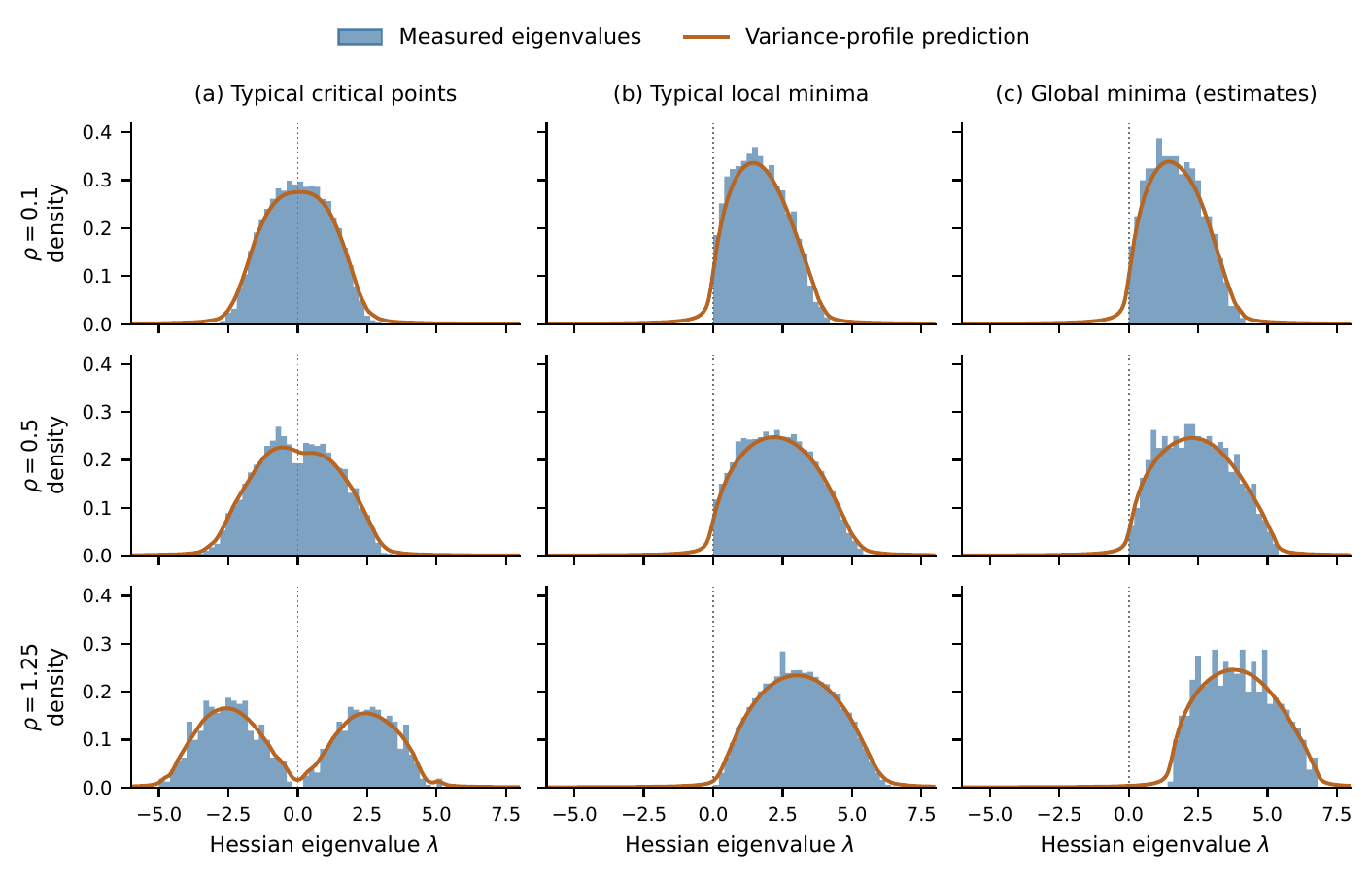
Blue histograms are measured Hessian eigenvalues and orange curves are the resolvent prediction. Columns: (a) typical critical points, (b) typical local minima, (c) lowest-energy minima found. Rows: $\rho=0.1$, $0.5$ and $1.25$. Dotted lines mark zero curvature. Broadening is $\eta=0.12$.

What to look at:

• Column (a), critical points. At weak locking ($\rho=0.1$) the spectrum is a single band straddling zero. As $\rho$ grows it widens and develops a dip at zero. By $\rho=1.25$ it has split into two bands centered near $\pm2\rho\approx\pm2.5$. This is the binary/quadrature separation, and the weight below zero matches $\langle k\rangle/N=1/2$.
• Column (b), typical minima. Everything is positive, as it must be for minima. At weak locking the spectrum still reaches almost to zero, so these minima are barely stable. More locking pushes the bulk to the right. The population itself changes with $\rho$, so the aggregate doesn’t translate perfectly rigidly the way a single binary state would.
• Column (c), lowest-energy minima. At weak locking they look much like the typical minima, crowding zero. At $\rho=1.25$ they are more clearly separated from zero than the typical minima. The trace identity above is consistent with that: lower energy means more mean curvature.

Across all nine panels the resolvent tracks the bulk well, using only the sampled phases and diagonal curvatures as input. The small orange tails beyond the histograms come from the finite broadening $\eta$, not from real eigenvalues. A tail crossing zero is therefore not a sign of instability.

A locking ramp

The paper also follows one trajectory under a linear ramp,

$$ \rho(t)=\rho_0+(\rho_f-\rho_0)\frac{t}{T}, $$

from $\rho=0$ to $1$ over $T=10$, tracking the phases, the energy, and the instantaneous Hessian spectrum (Fig. 2 in the paper). To avoid mistaking the locking offset for real progress, it tracks a shifted potential,

$$ \widetilde E=E+\frac{N\rho}{2}=-\sum_{i<j}J_{ij}\cos(\theta_i-\theta_j)+\rho\sum_i\sin^2\theta_i , $$

which equals the Ising energy $H$ exactly at a binary state.

The main caution: off equilibrium, the negative eigenvalues count directions of negative curvature, not the Morse index. Reaching all-positive curvature mid-trajectory does not mean the trajectory has converged. Once it does land on a binary minimum, more locking just slides that minimum’s spectrum to the right without changing the spins.

What this does and doesn’t show

What it shows:

• A cheap random-matrix model, fed only the diagonal curvatures and a phase-dependent variance, reproduces the bulk Hessian spectra of three quite different equilibrium populations.
• The binary/quadrature split explains why critical-point spectra separate into two bands, and why their average index is $N/2$.
• For binary states, locking acts as a pure spectral shift, and the local-field distribution sets the spectral shape.

What it doesn’t show:

• Correlations. The model ignores correlations that stationarity, stability and energy selection induce between the diagonal and the couplings. It describes the bulk conditionally, not the precise spectral edges.
• Sampling. The populations depend on the search procedure. The “global minima” are the lowest found, not certified optima.
• Basins. The attraction-domain estimates certify local convergence at fixed gains. They don’t give basin volumes or capture probabilities during a ramp.

The natural next step is the gap between the last two points: using the predicted spectral edge to say something about how large the certified neighborhoods are, population by population.